Description:
This tutorial is to demonstrate how to use the Graphical User Interface (GUI) to perform a regression using neural networks for one group of subjects with their structural data.
Each step will be illustrated with our example data. You can use your own data as well. See Tutorial_data_format_braph2 for how to prepare your structural data for BRAPH2.
- Start BRAPH 2 and select the Pipeline from the main GUI
Start MATLAB, go to the BRAPH2 folder, and run “braph2” with the following command:
>> braph2
Select “Pipeline Neural Networks Regression Structural Data” from the menu on the right-hand side. You can also use the search field by typing the keywords, e.g., Neural Networks Regression.
- Load a brain atlas from an XLS file
Press the button “Load a Brain Atlas XLS” (it is the only one that is active in the GUI) and select “desikan_atlas.xlsx” in the directory ./braph2/pipelines/structural NN /example data ST (MRI)/regression.
You can visualize the atlas by pressing “Plot the brain atlas” and play with the surface settings. Check the section Brain Atlas from our tutorial in Module 1 for how to control the appearance of this interface.
- Load subjects’ data
Press “Load Group ST from XLS” and select the data from one group of subjects at the directory ./braph2/pipelines/structural NN /example data ST (MRI)/regression/xls/ST_group.
- Dataset construction
Overall, this step decides the input for running the regression. Here, we use the structural data from the selected group.
Press “NN Dataset for Group” in the main pipelines GUI. For INPUT TYPE, select structural_data (this is the only option when using structural data). For TARGET NAME, set the variable as “age” to include in the regression. Here, our example includes age in the regression (Figure 1). After setting up INPUT TYPE and TARGET NAME, press “C” to create the dataset and move on to the next step.
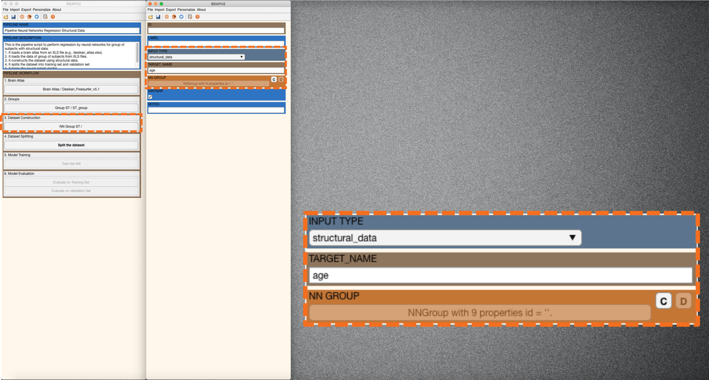
Figure 1. Regression of age using structural data.
- Dataset splitting
This step splits the data into a training set and a validation set.
Press “Split the Dataset” in the main pipeline GUI and an interface will be prompted for setting up the split (Figure 2). You can specify the index of the subjects who are assigned to the validation set (e.g., [2 3 5 7], meaning subject 2, subject 3, subject 5, and subject 7) or alternatively, you can type a number (between 0 and 1) that indicates the proportion of the subjects who are assigned to the validation set (e.g., 0.5, meaning half of the subject will be assigned to the validation set). We leave the default random indices (Figure 2). Finally, we press “C” in TRAINING GROUP and after “C” in VALIDATION GROUP to create the datasets (Figure 3).
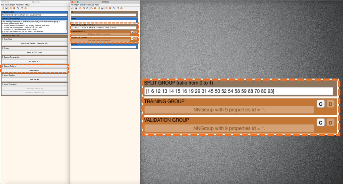
Figure 2. Specifying the index of subjects that will be assigned to the validation set.
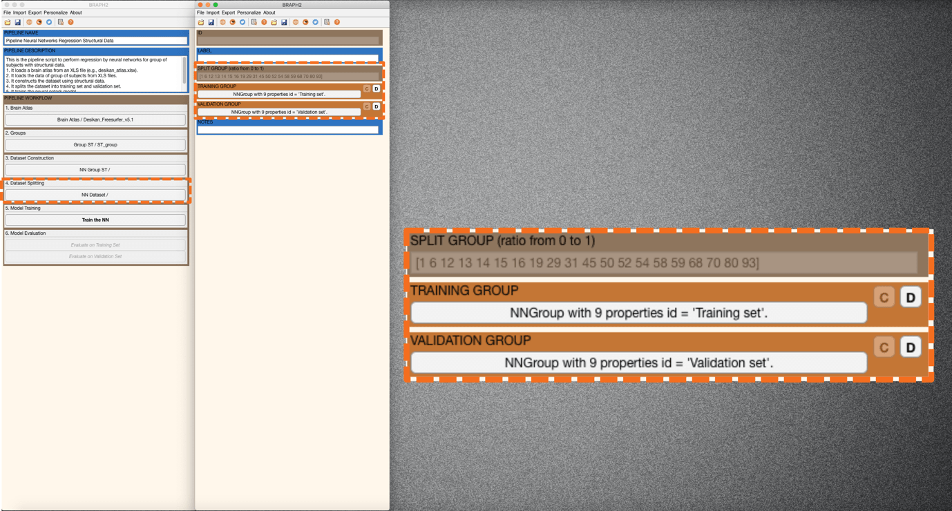
Figure 3. Splitting dataset into training set and validation set.
- Model Training
This step will train the neural network model with the specified parameters.
Press “Train the NN” in the main pipeline GUI and an interface will be prompted to set the options/parameters (LAYERS, BATCH, EPOCHS, SHUFFLE, SOLVER, FEATURE SELECTION PROPORTION, VERBOSE, PLOT TRAINING PROGRESS, PLOT LAYERS) for training neural networks (Figure 4 and Figure 5). Descriptions for each option/parameter are illustrated below:
LAYERS: This parameter specifies (i) how many fully connected layers are there and (ii) how many neurons are there in each layer as a vector. For instance, “[100 50]” means that there are two layers: 100 neurons for the first layer, and 50 neurons for the second layer.
(Note. In this case, each fully connected layer is followed by a dropout layer with a given dropout rate of 0.5.)
BATCH: This parameter specifies the size of the batch for each training iteration (as a positive integer). A batch is a subset of the training set and is used to (i) evaluate the gradient of the loss function and (ii) update the weights.
EPOCHS: This parameter specifies the maximum number of epochs for training (as a positive integer). An epoch is the full pass of the training algorithm over the entire training set.
SHUFFLE: This parameter specifies the option for data shuffling. There are three options: “once”, “never”, and “every-epoch”. “once” means to shuffle the training and validation data once before training. “Never” means not to shuffle the data at all. “Every-epoch” means to shuffle the training data before each training epoch.
SOLVER: This parameter specifies the option of solver. There are three options: “sgdm”, “rmsprop”, and “adam”. “sgdm” uses the stochastic gradient descent with momentum (SGDM) optimizer. “rmsprop” uses the RMSProp optimizer. “adam” uses the Adam optimizer.
FEATURE SELECTION PROPORTION: This parameter specifies the proportion of the features to be selected for training the neural networks. All the features are analyzed and given individual scores based on the mutual information analysis. Based on the scores, all the features can be ranked, and the user can set a proportion for including part of the ranked features that are relatively informative.
VERBOSE: This parameter indicates whether to display training progress information in the command window.
PLOT TRAINING PROGRESS: This parameter indicates whether to create a figure and displays training metrics at every iteration.
PLOT LAYERS: This parameter indicates whether to create a figure to display the neural network architecture.
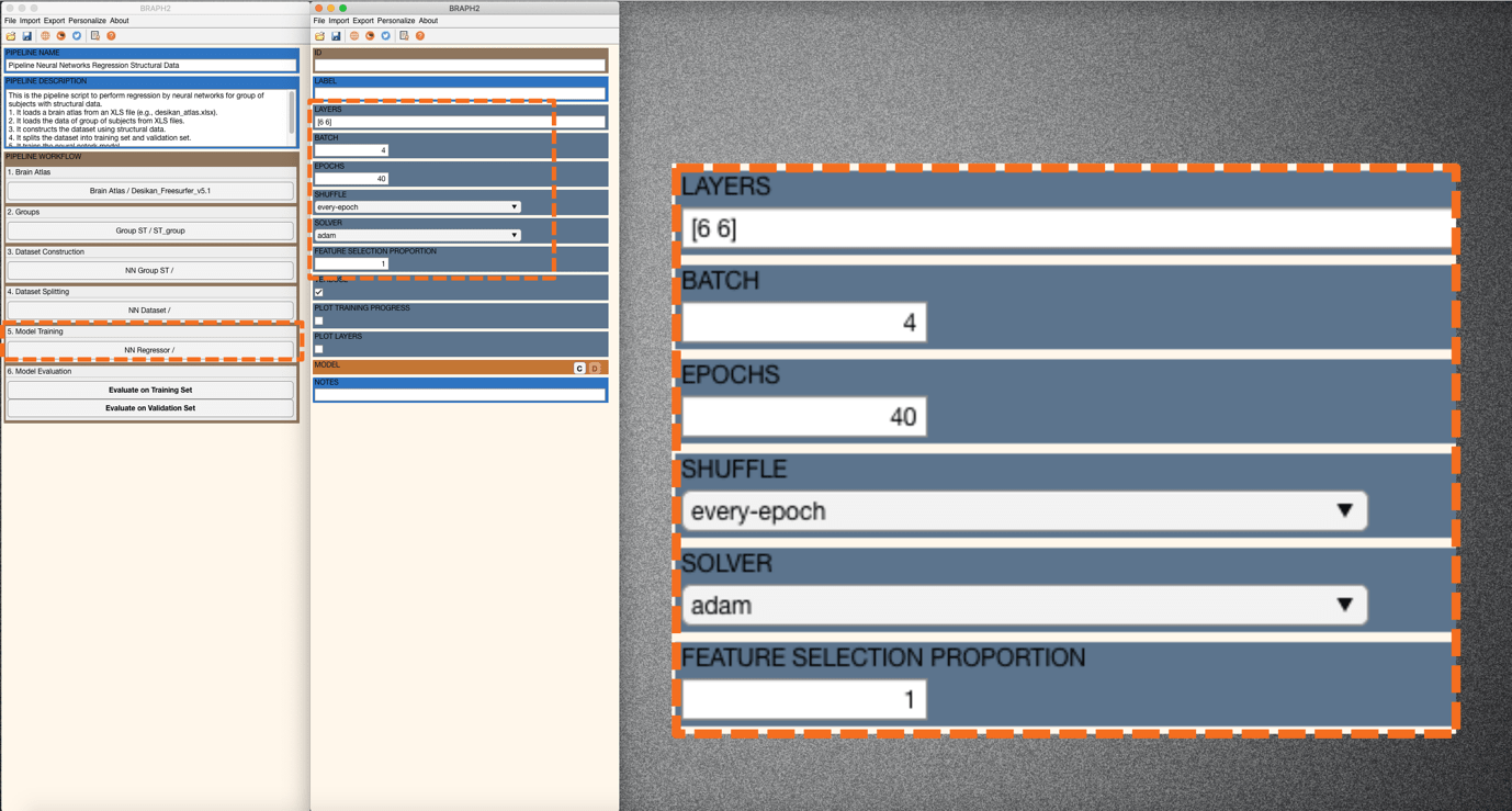
Figure 4. Setting the parameters for training neural networks.
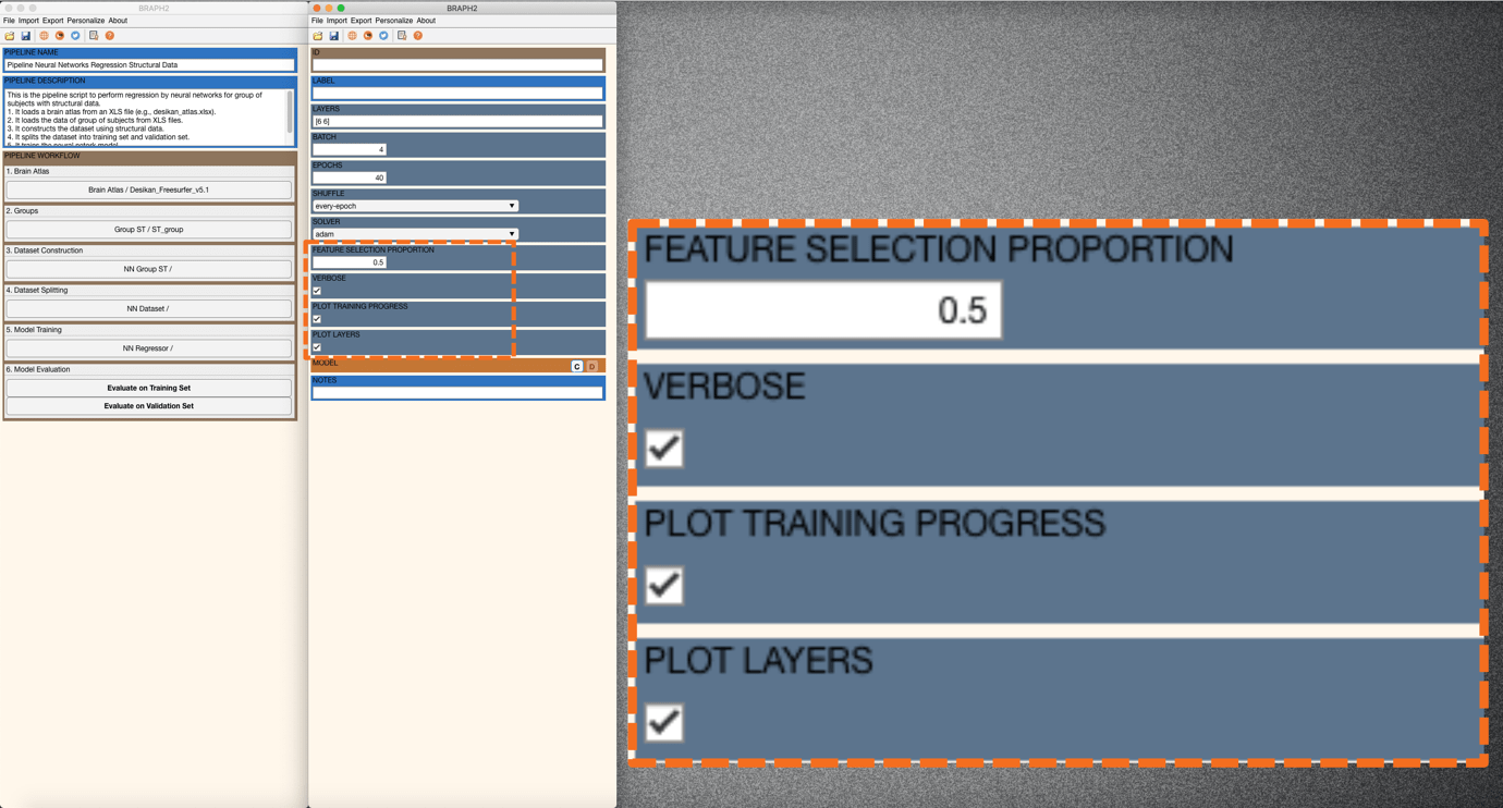
Figure 5. Changing FEATURE SELECTION PROPORTION to 0.5 and selecting the different plot options.
After changing the FEATURE SELECTION PROPORTION to 0.5 and checking VERBOSE, PLOT TRAINING PROGRESS, and PLOT LAYERS (Figure 5), you can now train the model by clicking on the “C” in MODEL. In this example, you will see a plot of layers, a plot of training progress, and the verbose in the command line window (Figure 6).
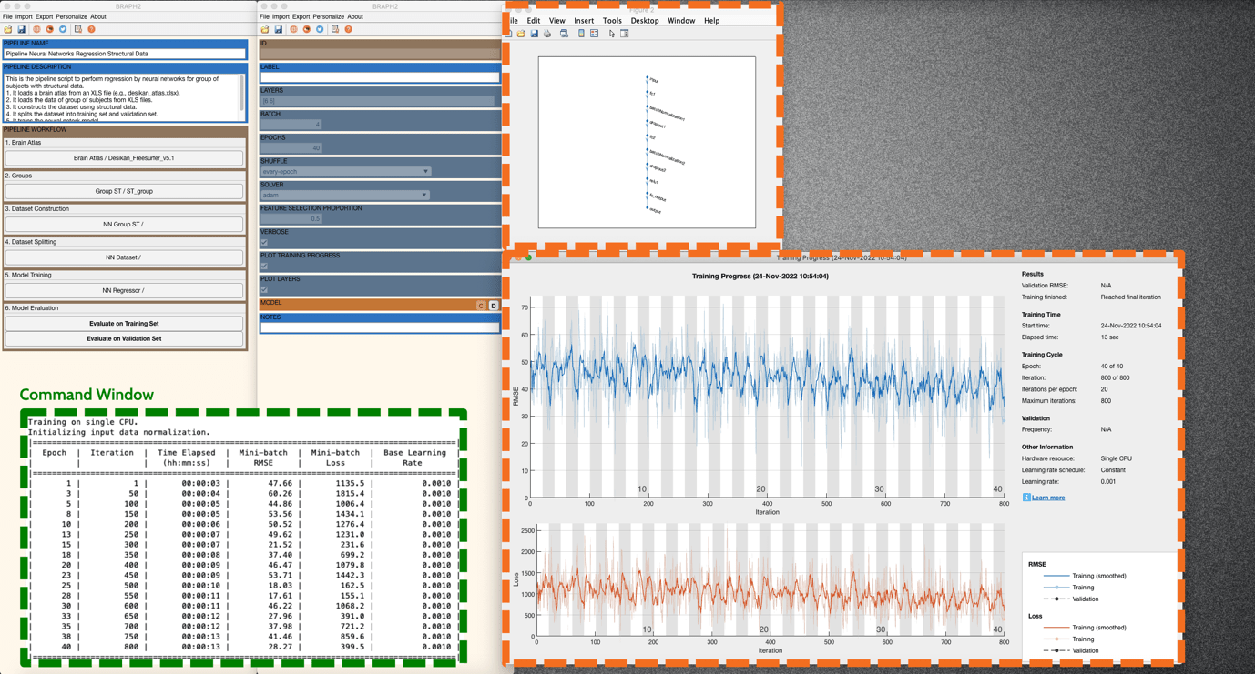
Figure 6. The plots for the options VERBOSE, PLOT TRAINING PROGRESS, and PLOT LAYER.
- Model Evaluation
This step evaluates the performance of the neural network model on the training set and the validation set.
Press “Evaluate on Training Set” in the main pipeline GUI and an interface will be prompted to calculate GROUP WITH NN PREDICTION, RMSE, and SCATTER CHART (Figure 7).
In GROUP WITH NN PREDICTION, you can get a group of subjects that convey the prediction from the trained neural networks.
In RMSE, you can get the root mean square error, a measure to evaluate the model’s predictions when compared to actual target values (here, age).
A SCATTER CHART lists all the predictions and targets from all subjects in this group. For PFSP, press “Plot” and a scatter plot of the targets for the predictions will be prompted (Figure 8). You can adjust the figure with the settings panel.
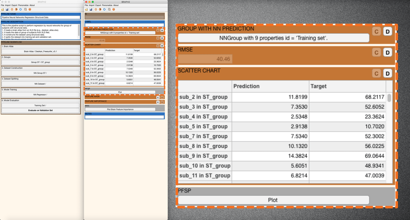
Figure 7. RMSE calculation and SCATTER CHART listing all predictions and targets from all subjects.
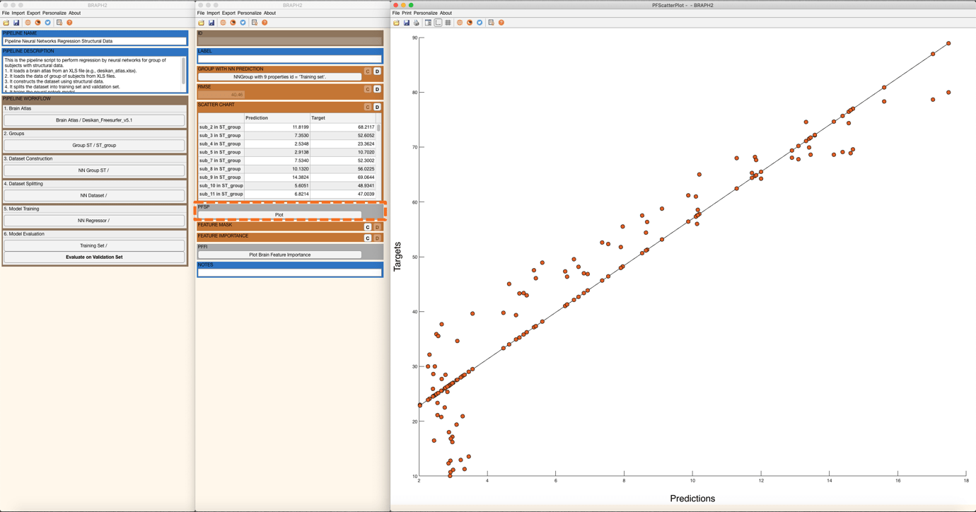
Figure 8. A scatter plot of the targets with respect to the predictions.
Now, it is time to calculate the feature mask. The Feature Mask indicates which features are selected to train/test the model. In our example, half of the feature mask is shown as zeros, and the other half is shown as ones. It is because the FEATURE SELECTION PROPORTION has been set as 0.5, meaning only half of the features are selected to train/test the model. More interestingly, we can calculate the Feature Importance (Figure 9). After pressing the “C” in FEATURE IMPORTANCE to calculate the feature importance, we can further visualize the feature importance on a brain surface.
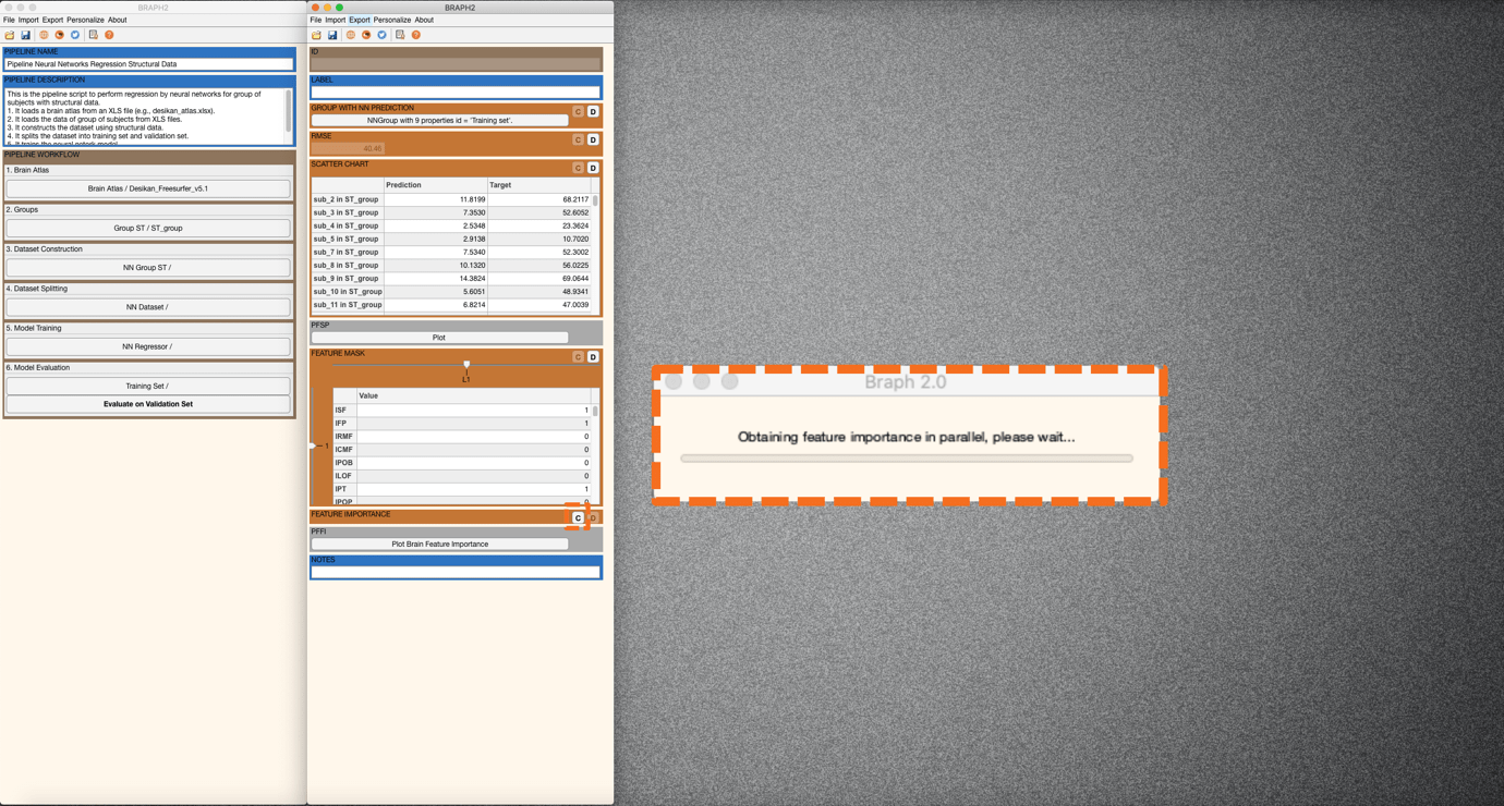
Figure 9. Obtaining feature importance on the training set.
To check the feature importance on a brain surface, you can right-click on “Plot Brain Feature Importance” (Figure 10). A new figure with the brain surface will be prompted for brain region visualization (all with default settings). For further adjustments, go to settings and scroll down in the Settings panel. You will find Measure and please tick on the box. Now, the color and size of all spheres will be adapted in proportion to the feature importance’s value, where blueish colors represent smaller values, and red larger (Figure 10).
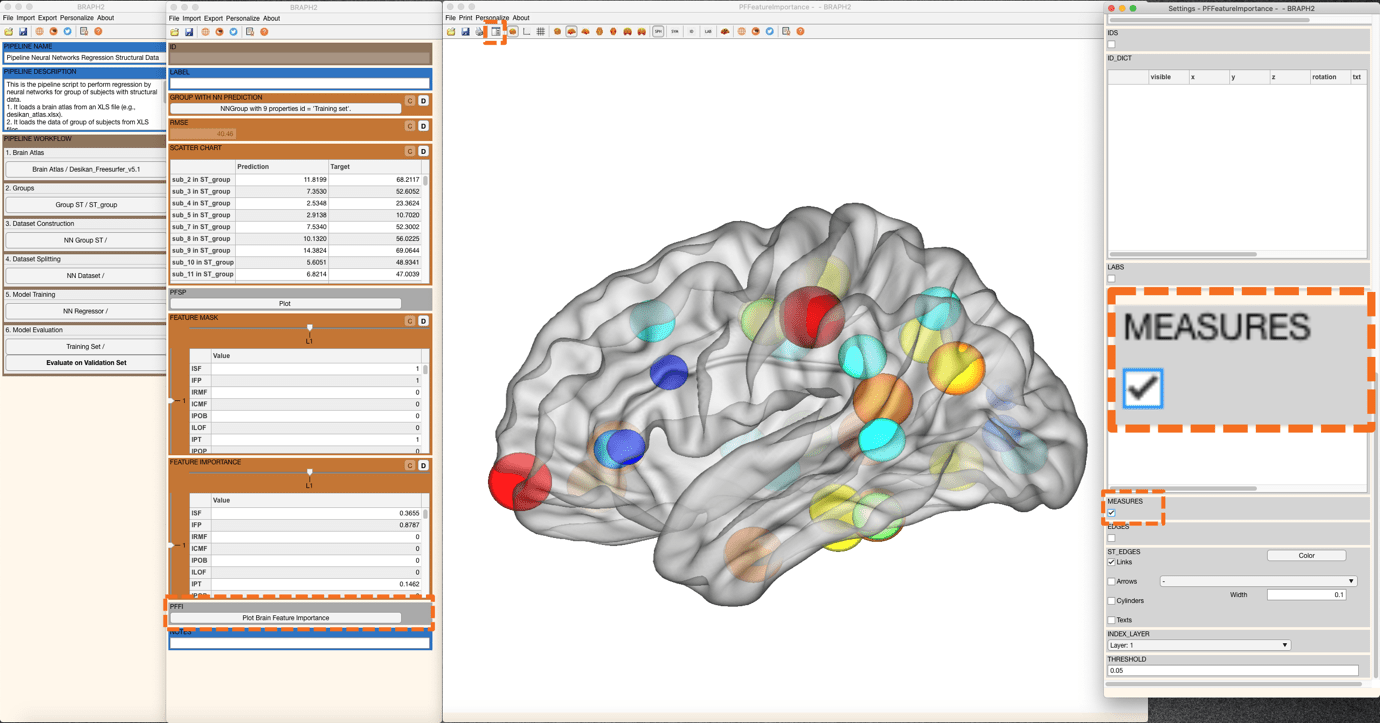
Figure 10. Visualization of feature importance on the training set.
Now, to evaluate the performance on the validation set, press “Evaluate on Validation Set” in the main pipeline GUI and similarly to the previous step obtain the RMSE, SCATTER CHART, FEATURE MASK, and FEATURE IMPORTANCE (Figure 11 and Figure 12).
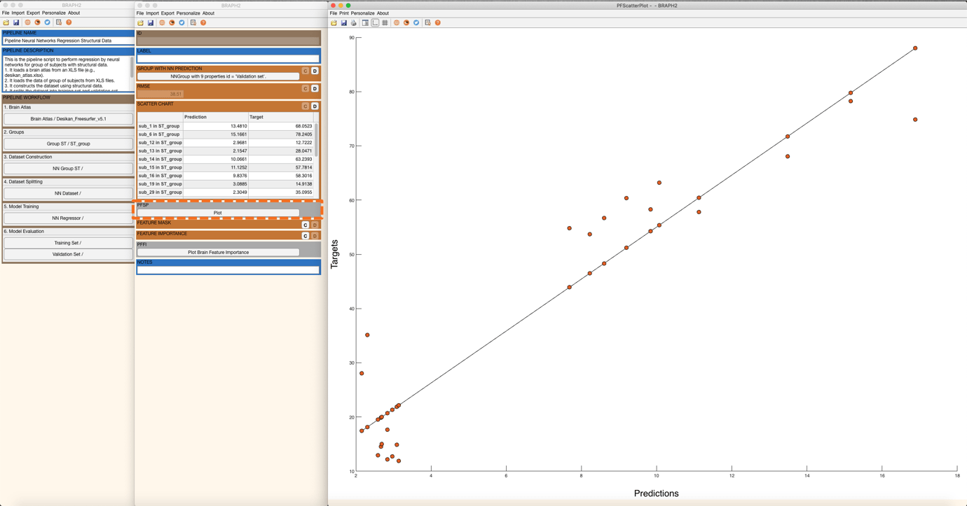
Figure 11. Scatter plot for targets and predictions for the validation set.
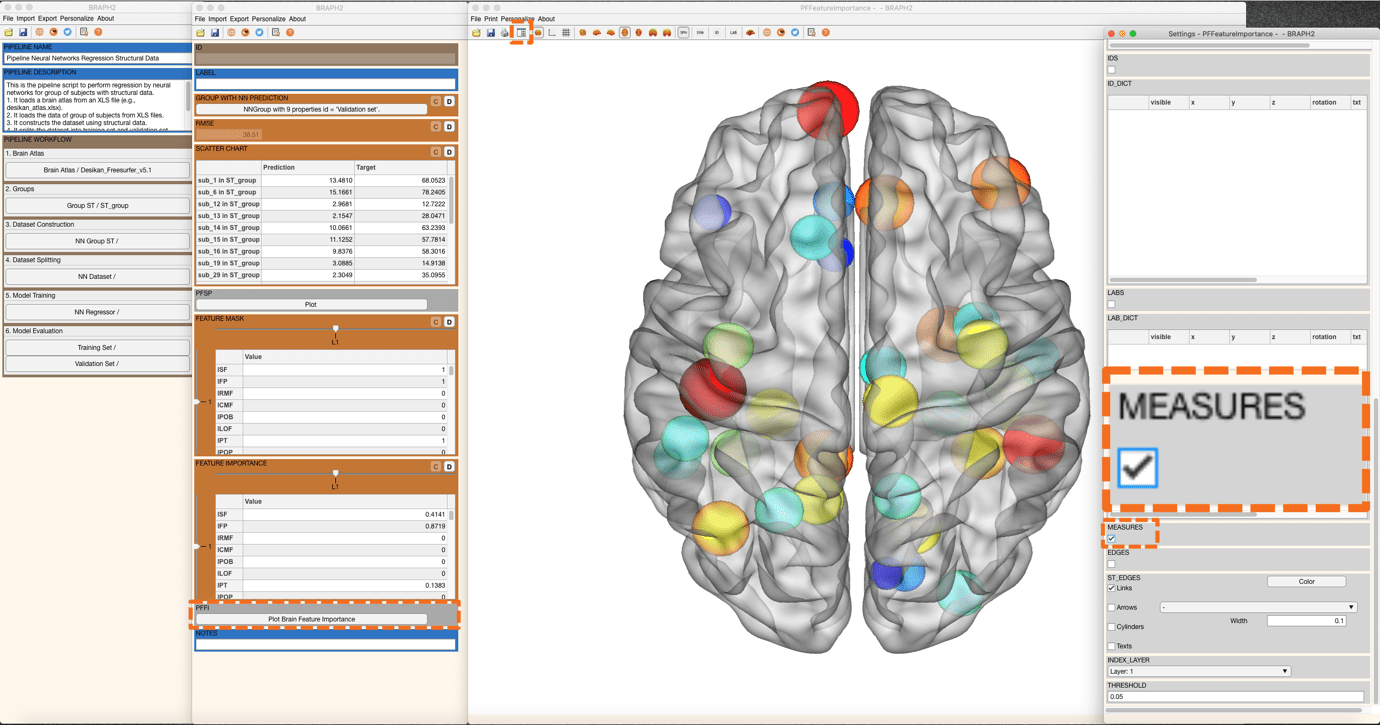
Figure 12. Visualization of feature importance on the validation set.