Description:
This tutorial is to demonstrate how to use the Graphical User Interface (GUI) to perform a classification using neural networks for two groups of subjects with their connectivity data and weighted undirected graphs.
Each step will be illustrated with our example data. You can use your own data as well. See Tutorial_data_format_braph2 for how to prepare your structural data for BRAPH2.
- Start BRAPH 2 and select the Pipeline from the main GUI
Start MATLAB, navigate to the BRAPH2 folder, and run “braph2” with the following command:
>> braph2
Select the Pipeline Neural Networks Classification Connectivity WU in the right menu. You can use the search field, typing Neural Networks Classification for example.
- Loading a brain atlas from an XLS file
The first step is to load a brain atlas from an XLS file. Press the button “Load a Brain Atlas XLS” (the only one active in the pipeline GUI) and then select the desikan_atlas.xlsx in the directory ./braph2/pipelines/connectivity NN/example data CON (DTI)/classification.
Finally, you can visualize the atlas by pressing “Plot the brain atlas” and playing with the surface settings. Check the Brain Atlas section from the tutorial of module 1 for more information on how to control the appearance of this interface.
- Loading the subject’s group data
To load the data for the two groups you would like to compare press “Load Group CON 1 from XLS” and select the folder for subjects of Group1 which is at the directory ./braph2/pipelines/connectivity NN/example data CON (DTI)/classification/xls/GroupName1. After, load the data for Group 2 which can be found at the directory ./braph2/pipelines/connectivity NN/example data CON (DTI)/classification/xls/GroupName2.
- Dataset Construction
In this step we decide the input to use for the classification. In this case, we can choose between using adjacency matrices or graph measures.
To construct the dataset for the first group press “NN Dataset for Group 1” which will open a GUI to select the type of input data (adjacency matrices or graph measures, Figure 1).
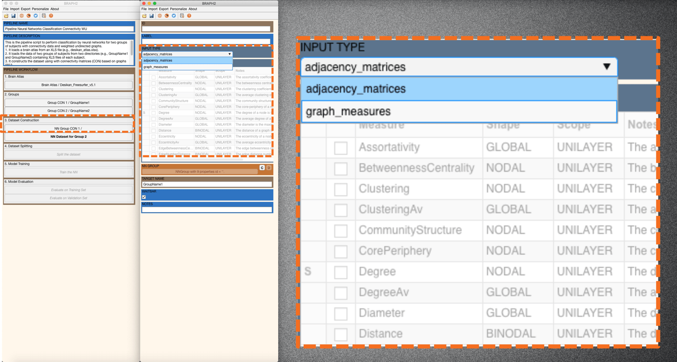
Figure 1. Options for INPUT TYPE.
We select graph measures as input, and then from the measures list we select Strength and Clustering measures and press “Set selected measures” to set them as input measures to be used (Figure 2), and finally, we press “C” in NN GROUP panel to create the dataset (Figure 3). Note that when the measure is set successfully, an S appears on its left.
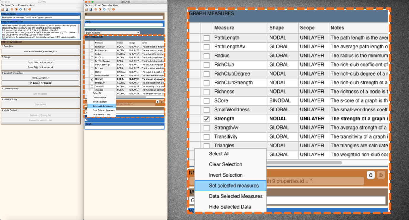
Figure 2. Set selected measures.
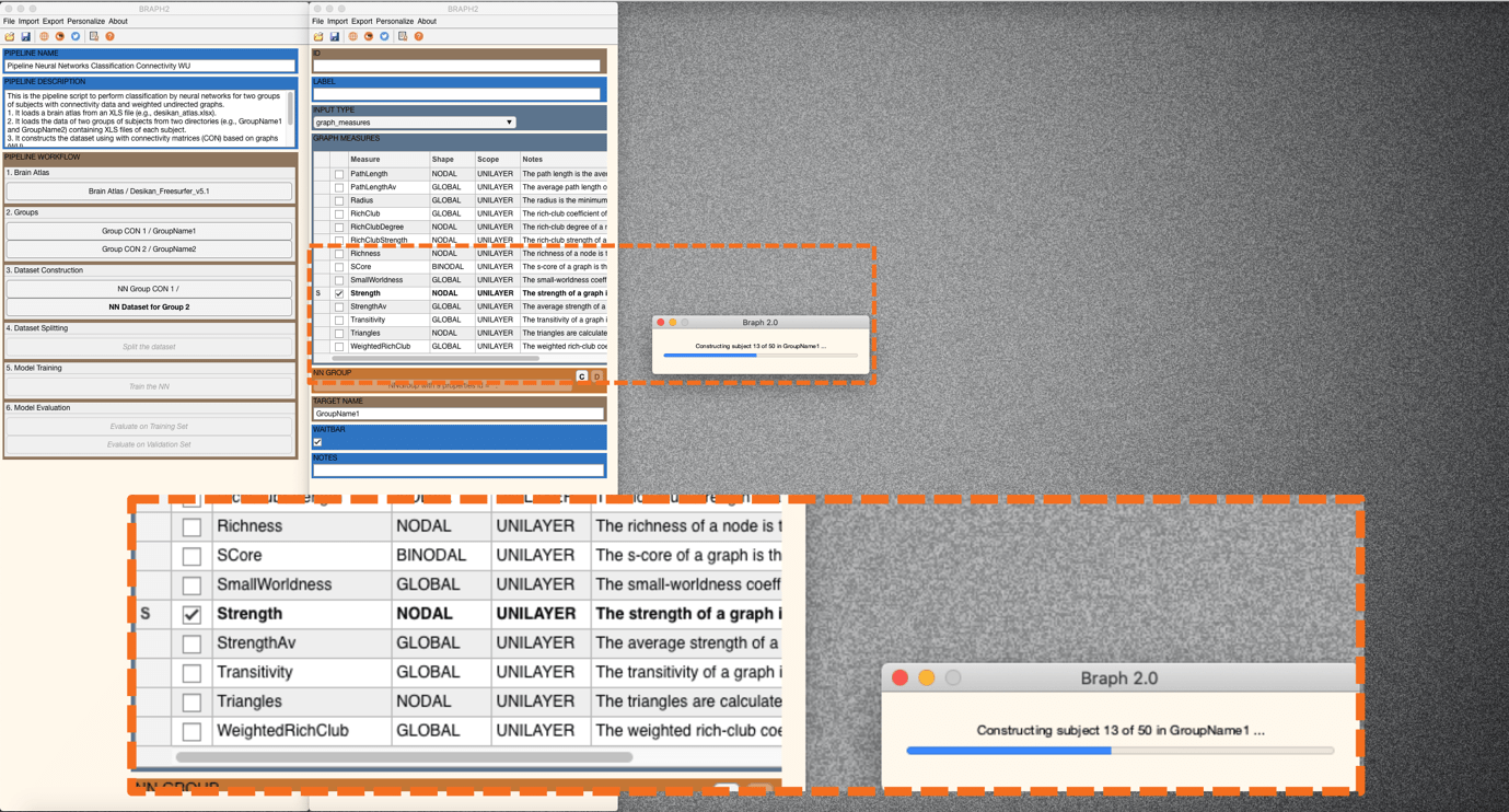
Figure 3. Constructing the dataset with selected graph measures.
For group 2, you will see that the same measures have been set in the measure list as of group 1, thanks to the callback function in braph2 (Figure 4). We can then construct the dataset for group 2 accordingly by pressing “C” in NN GROUP.
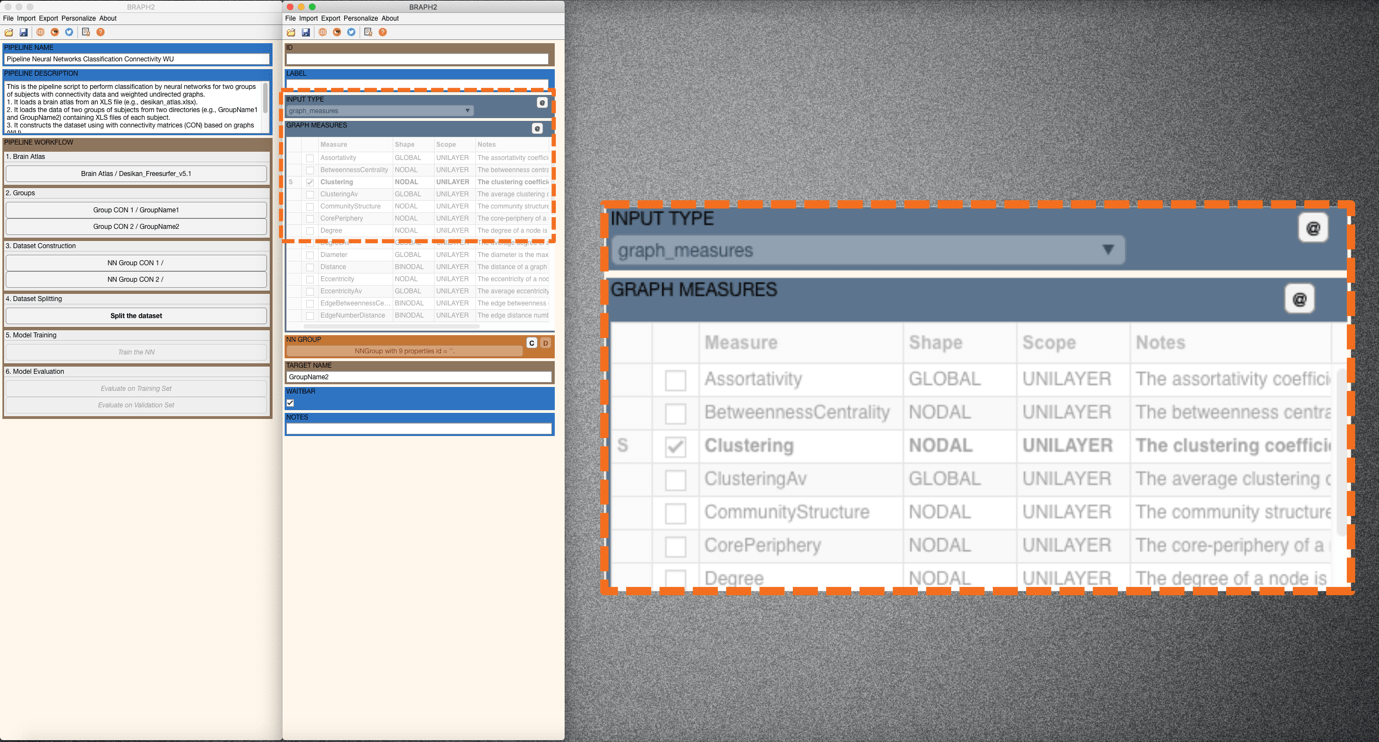
Figure 4. Constructing the dataset with selected graph measures for group 2.
- Dataset Splitting
In this step, we divide the data into a training set and a validation set.
The next step is splitting the data into training and validation sets, for that press “Split the Dataset” in the main pipeline GUI. An interface will be opened (Figure 5) where we can set the SPLIT GROUP 1 and SPLIT GROUP 2. We can specify the index of the subjects that are assigned to the validation set (e.g. [9 16 42 44 48], meaning subject 9, subject 16, subject 42, subject 44, and subject 48 to be in the validation group). Alternatively, we can also type a number (between 0 and 1) that indicates the proportion of the subjects to be in the validation set (Figure 6). Here, we set to 0.1 the proportion of validation set in both groups (Figure 5). Finally, we press “C” in TRAINING GROUP and after “C” in VALIDATION GROUP to create the datasets (Figure 6).
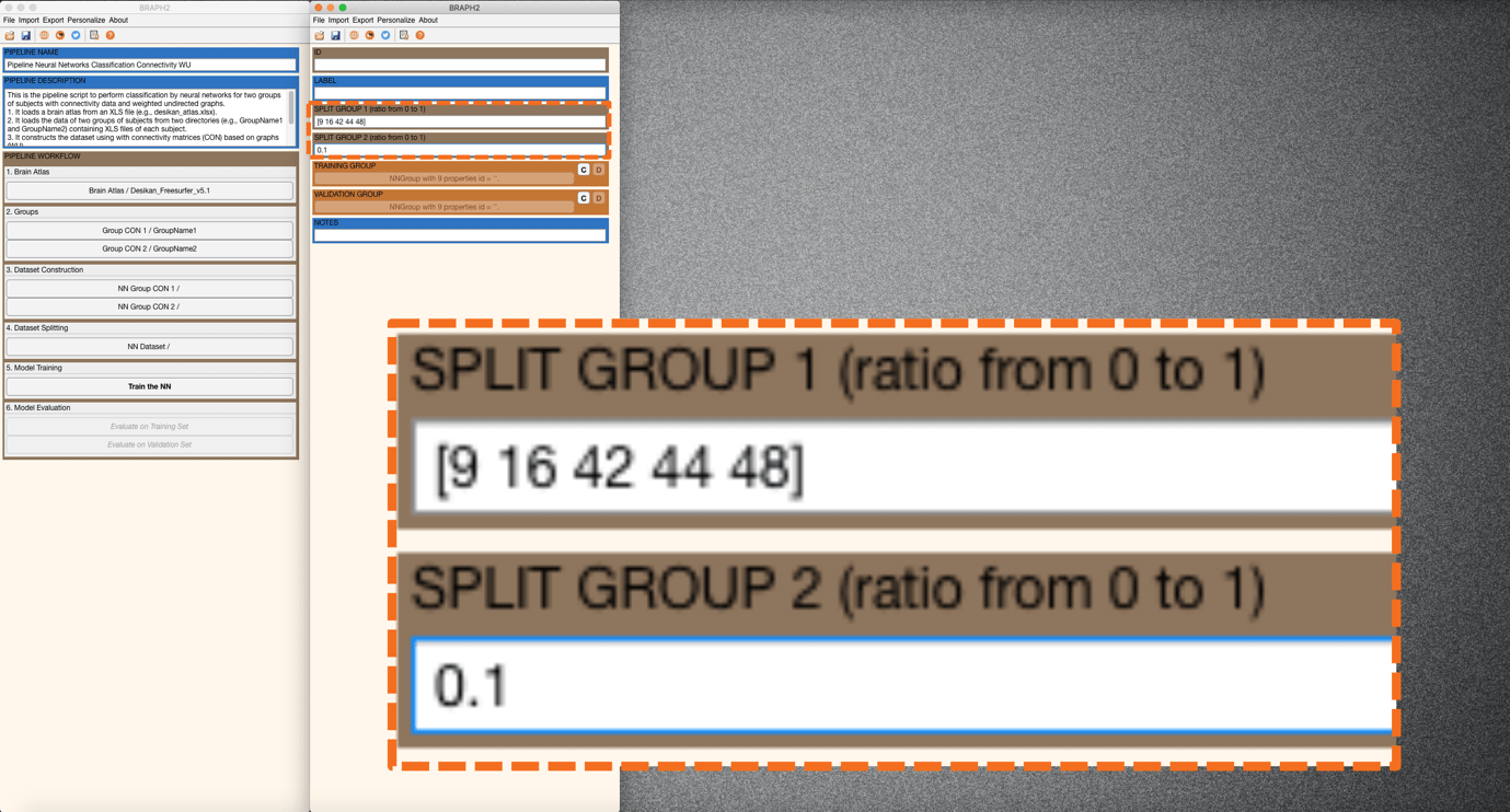
Figure 5. Specifying the index of subjects or the proportion of all subjects to be assigned in the validation set.
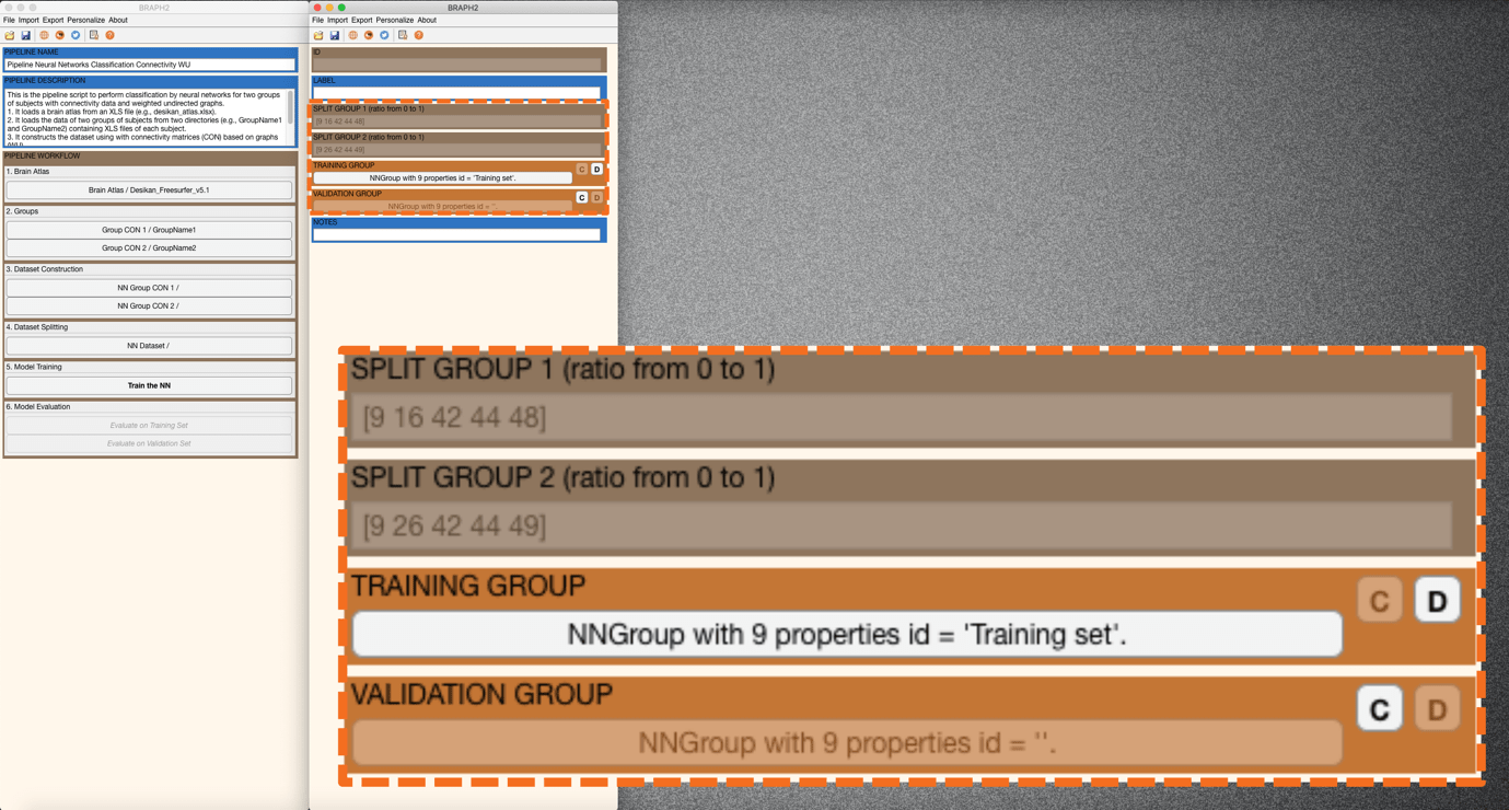
Figure 6. Splitting the dataset into the training set and validation set
- Model Training
This step will train the neural network model with the specified parameters.
Press “Train the NN” in the main GUI and an interface will be prompted to set the options/parameters (LAYERS, BATCH, EPOCHS, SHUFFLE, SOLVER, FEATURE SELECTION PROPORTION, VERBOSE, PLOT TRAINING PROGRESS, PLOT LAYERS) for training neural networks. Descriptions for each option/parameter are illustrated below:
LAYERS: This parameter specifies (i) how many fully connected layers are there and (ii) how many neurons are there in each layer as a vector. For instance, “[100 50]” means that there are two layers: 100 neurons for the first layer, and 50 neurons for the second layer.
(Note. In this case, each fully connected layer is followed by a dropout layer with a given dropout rate of 0.5.)
BATCH: This parameter specifies the size of the batch for each training iteration (as a positive integer). A batch is a subset of the training set and is used to (i) evaluate the gradient of the loss function and (ii) update the weights.
EPOCHS: This parameter specifies the maximum number of epochs for training (as a positive integer). An epoch is the full pass of the training algorithm over the entire training set.
SHUFFLE: This parameter specifies the option for data shuffling. There are three options: “once”, “never”, and “every-epoch”. “once” means to shuffle the training and validation data once before training. “Never” means not to shuffle the data at all. “Every-epoch” means to shuffle the training data before each training epoch.
SOLVER: This parameter specifies the option of solver. There are three options: “sgdm”, “rmsprop”, and “adam”. “sgdm” uses the stochastic gradient descent with momentum (SGDM) optimizer. “rmsprop” uses the RMSProp optimizer. “adam” uses the Adam optimizer.
FEATURE SELECTION PROPORTION: This parameter specifies the proportion of the features to be selected for training the neural networks. All the features are analyzed and given individual scores based on the mutual information analysis. Based on the scores, all the features can be ranked, and the user can set a proportion for including part of the ranked features that are relatively informative.
VERBOSE: This parameter indicates whether to display training progress information in the command window.
PLOT TRAINING PROGRESS: This parameter indicates whether to create a figure and displays training metrics at every iteration.
PLOT LAYERS: This parameter indicates whether to create a figure to display the neural network architecture.
Here we leave the default options for SHUFFLE and SOLVER and the rest of the parameters.
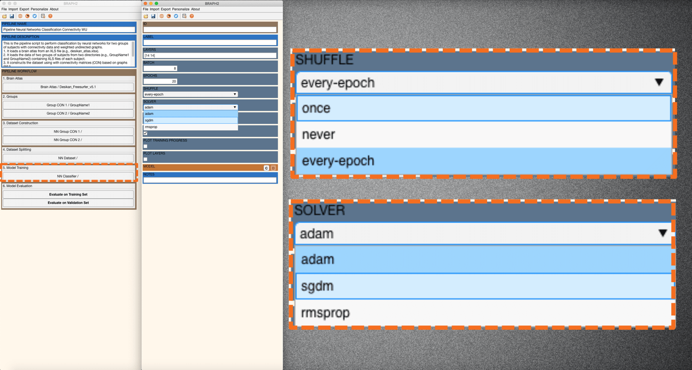
Figure 7. Different options for shuffle and solver. We leave the default options.
- Model Evaluation
In this step, we evaluate the performance of the neural network model on the training set as well as on the validation test.
After training the model we evaluate its performance. First, we evaluate the performance of the training set by pressing “Evaluate on Training Set” in the main pipeline GUI. An interface will open, and we can calculate GROUP WITH NN PREDICTION, AUC, and CONFUSION MATRIX (Figure 8).
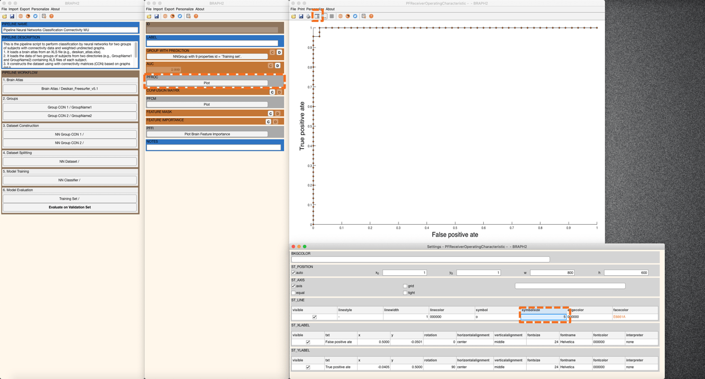
Figure 2.8. Plot of receiver operating characteristic curve.
In GROUP WITH NN PREDICTION, one can get a group in which subjects convey the prediction from the trained neural networks. In AUC, one can get the area under the receiver operating characteristic, a measure to evaluate the model’s performance when compared to actual target values. We can also plot of ROC curve by pressing PFROC (Figure 8). You can also adjust the figure with the settings panel (Figure 8).
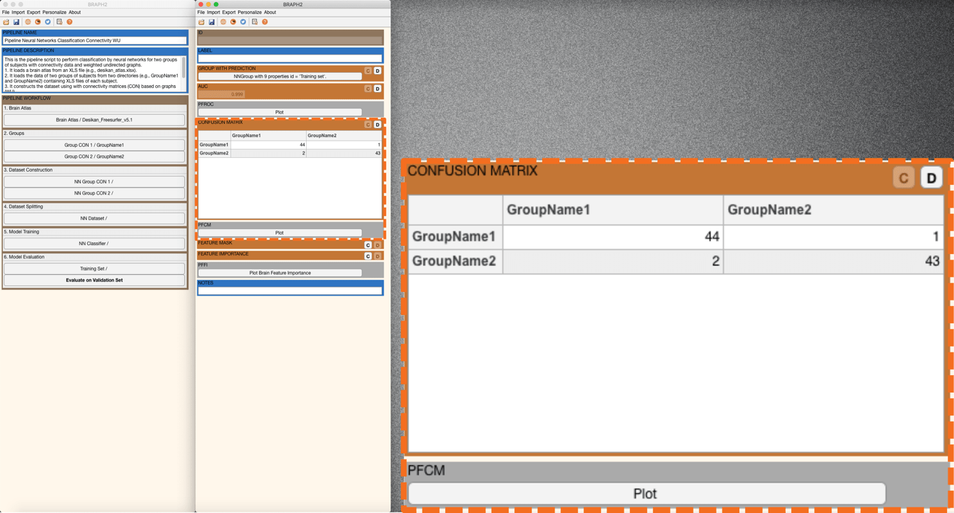
Figure 9. Plot of the confusion matrix
In CONFUSION MATRIX, one can get the confusion matrix determined by the target and predicted groups. Press the plot button in PFCM to plot the confusion matrix (Figure 9).
Now it is time to calculate the feature mask. We calculate the FEATURE MASK to get a mask that indicates which features are selected for training the model (Figure 10). In this case, we can see all values in the features mask are one, because we set FEATURE SELECTION PROPORTION to 1.0, which means all features are selected to train neural networks. Note that feature importance analysis does not apply when the input is composed of graph measures.
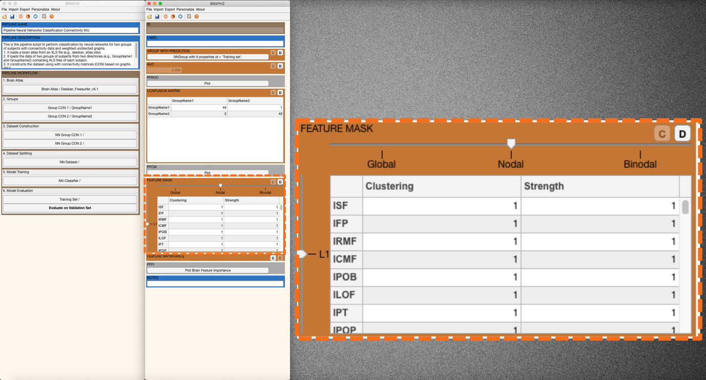
Figure 10. Feature mask indicating which features are selected to train neural networks
Finally, we can evaluate the performance of the validation set, by pressing “Evaluate on Validation Set” in the main pipeline GUI and following the same steps as in the training evaluation to obtain the AUC, CONFUSION MATRIX, and FEATURE MASK (Figure 11).
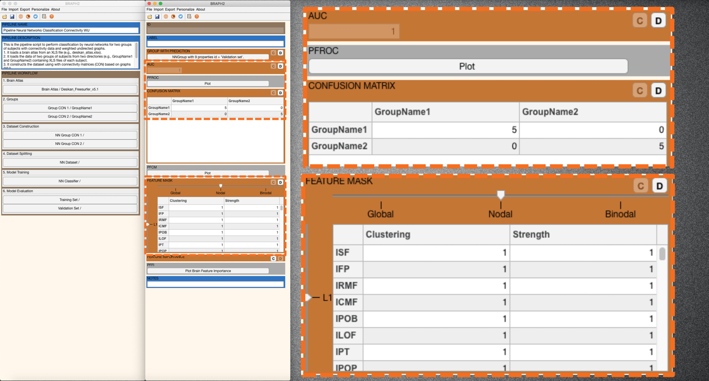
Figure 11. Evaluation of the validation set.