FUN Comparison BUD
Description:
This is the Graphical User Interface (GUI) tutorial for the pipeline that compares two groups of subjects using functional data (such as fMRI) and binary undirected graphs at fixed densities.
In this tutorial, we will use the example data, but you can use your own data as well (for instructions on how to prepare your own functional data to be analyzed in BRAPH2, see tutorial Functional Data format).
- Start BRAPH 2 and select the Pipeline from the main GUI
Start MATLAB, navigate to the BRAPH2 folder and run “braph2” with the following command:
>> braph2
Select the Pipeline Functional Comparison BUD in the right menu. You can use the search field, typing functional for example (Figure 1).
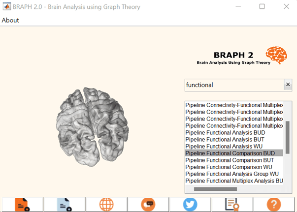
Figure 1. Landing GUI.
Once you click on the pipeline, the window on Figure 2 will open.
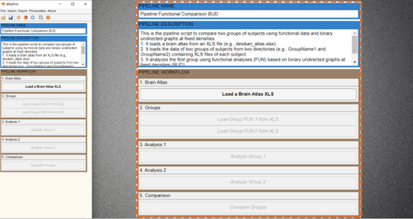
Figure 2. Landing pipeline GUI
- Loading a brain atlas from an XLS file
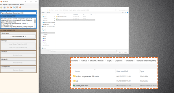
Figure 3. Loading an atlas file.
The first step is to load a brain atlas from an XLS file. Press the button “Load a Brain Atlas XLS” (the only one active in the pipeline GUI, Figure 2) and then select the aal90_atlas.xlsx in the directory ./braph2/pipelines/functional/example data FUN (fMRI) (Figure 3).
Finally, to visualize the atlas press “Plot the brain atlas” and play with the surface settings (Figure 4). Check the Brain Atlas for more information on how to control the appearance in this interface.
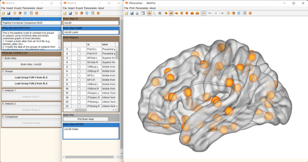
Figure 4. Plot the brain atlas.
- Loading subject’s data for each group
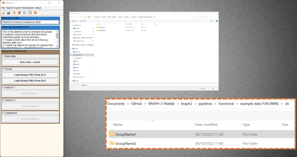
Figure 5. From the pipeline GUI, first load data for group 1 (GroupName1) and then for group 2.
To load the data for the two groups you would like to compare press “Load Group FUN 1 from XLS” and select the folder for subjects of Group1 which is at the directory ./braph2/pipelines/functional/example data FUN (fMRI)/xls/GroupName1 (Figure 5). After, load the data for the group 2 which can be found at directory ./braph2/pipelines/functional/example data FUN (fMRI)/xls/GroupName2.
- Performing the functional analysis of group 1
Analysis of the first group using functional analyses (FUN) based on binary undirected graphs at fixed densities (BUD).
First press “Analyze Group 1” to open the interface for its analysis (Figure 6). In this interface, you can specify the parameters for constructing the graph from the time series of fMRI data (type of correlation, and what to do with the negative weights). Especially, in the densities section, you can specify the densities, in this case we will use the values “[20 25 30]” or “20:5:30”. Then under GRAPHS section, by pressing “C” you can check the graphs for each subject. What more interesting would be to plot the average graph for the whole group, for that go to section GRAPH MEASURES and press “C”, right click on the left of a measure to deploy the menu seen on Figure 7 and select “Plot Graph”. We will see an adjacency graph on the right, which is the graph from the first density (in our case, density of 20) and from the first subject.
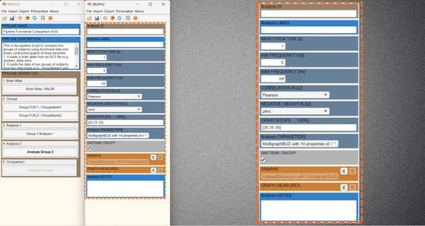
Figure 6. After pressing Analyze group 1, interface for Analysis of group 1 opens.
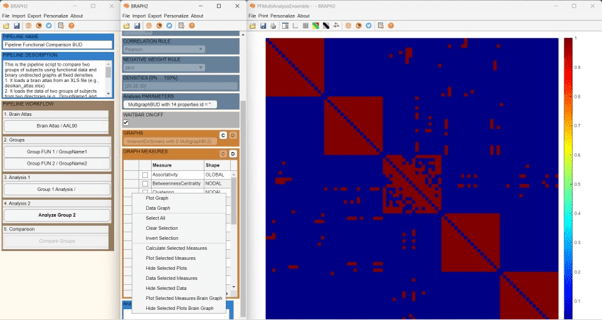
Figure 7. Plot graph. By default, we see the adjacency matrix at the first density (in this case density of 20).
Press the settings panel button in Figure 8, the settings panel will show up. In the last section “DT” of the settings panel, we can select at which density to show the adjacency matrix. Moreover, in the section “G”, we can select to plot the Mean Graph for the group or the individual graphs.
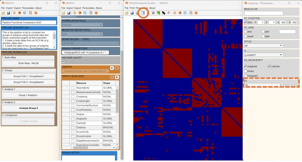
Figure 8. Plot graph at a fixed density.
Now it is the moment to calculate some connectivity measures for group 1. Select one measure, for example, Degree (nodal), and calculate by right clicking on the left-side of the measures list and press “Calculate Selected Measures”. When the measure is calculated, a C appears on its left, and now, again by right clicking on the left-side of the measures list and pressing “Plot Selected Measures Brain Graph” (see Figure 9), we will be able to visualize the results of Degree for group 1.
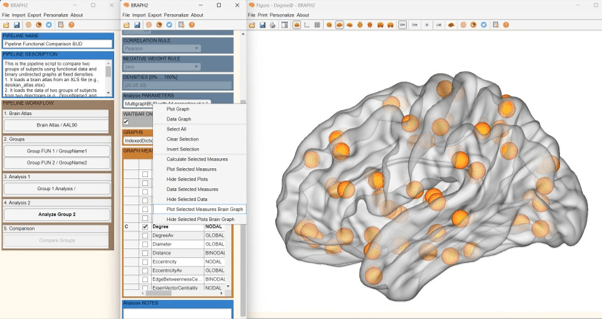
Figure 9. When the measure is calculated, the C appears and then you can plot it on a brain surface.
A new figure with the brain surface will open with default settings for brain region visualization (Figure 10). If we go to settings, we go down in the Settings figure, we will find Measures and EDGES panels. By checking the boxes, the link will appear, and the size of all spheres will be adapted in proportion to the measure’s value, where blueish colors represent smaller values, and red larger.
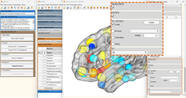
Figure 10. Selecting the check box at Measures and Edges.
We can also first press “Data Selected Measures” from the same menu mentioned earlier, and then a figure will open showing the array of values for the measure (Figure 11), and from there we can press “Plot Brain Multi Graph” to visualize the results of Degree for group 1 on a brain surface.
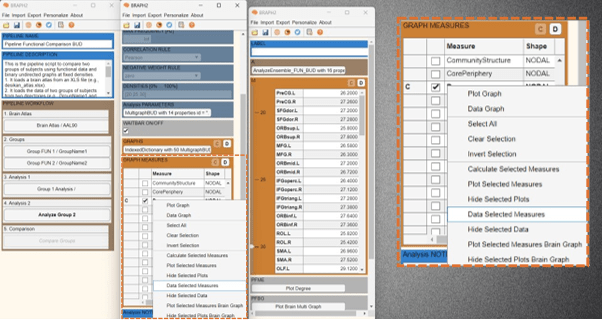
Figure 11. Show the data of the selected measure.
- Performing the functional analysis of group 2
Analysis of the second group using the same parameters selected for the first group (functional analyses (FUN) based on binarized undirected graphs at fixed densities (BUD)).
Follow the previous steps in the analysis of group 1 and explore some other measures for group 2.
- Comparing the two groups
To proceed with the group comparison press “Compare Groups” and the interface to select the comparison parameters will open (Figure 14). After setting the desired permutation number (recommended 1000 – 10000 permutations), press “C” under the ENSEMBLE COMPARISONS section to open the list of measures to use to compare the groups.
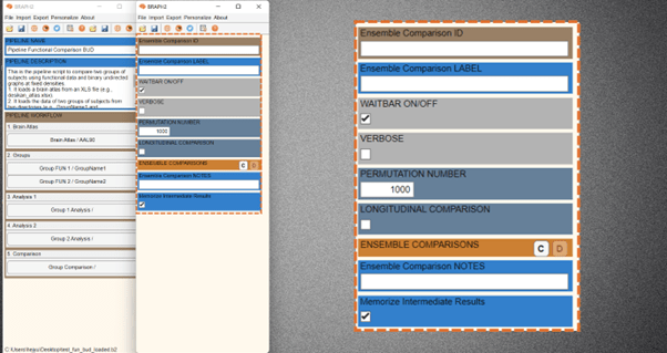
Figure 12. Open the Group Comparison interface.
It is possible to select multiple measure to be compared, and then right click on the left of the measure table and select “Calculate Selected Comparisons” (Figure 13). Depending on how many permutations you use it will take less or more time.
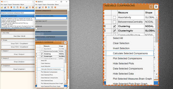
Figure 13. Calculation of the comparison.
Once the calculations are done, you should see a C on the left of the measure to be compared (Figure 13). Then press “Data Selected Comparison” to show the difference values between groups and the associated p-values resulting from the permutation testing (Figure 14). Significant differences after FDR correction at the value of q = 0.05 (q level can be changed at the panel QVALUE) are highlighted in the table by green for 25% of density (density can be changed by the sided slider in the panel DIFF) (Figure 15).
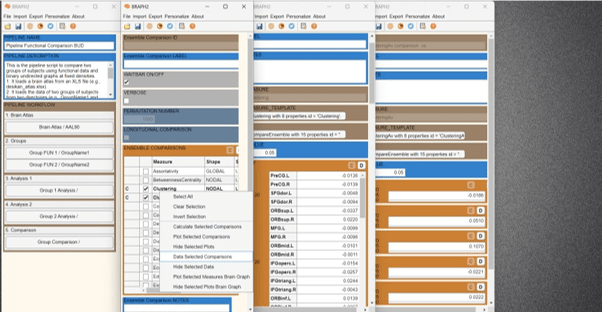
Figure 14. Show the results of the comparisons of multiple measures.
Also, you can add the data from other important variables like the p-values resulting from the permutation testing, by editing the layout (Go to “Personalize” and then check the box of variables to be shown) (Figure 15).
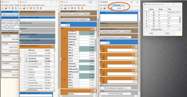
Figure 15. Show the results of the comparisons of multiple measures.
We can then plot the results of a nodal measure (in this case, Clustering) from the comparison by pressing “Plot Brain Multi Graph” in the measure’s table GUI (Figure 16). A new figure with the brain surface will open with default settings for brain region visualization. If we go down in the Settings figure, we will find MEASURES, FDR SHOW, QVAL, and DT panels. By checking the boxes and changing the density to one density of interest, for example 25%, just the regions that are significantly different between groups after applying FDR correction at the desired level (in the Figure 16, q value is set at 0.005) will be shown, and the rest will be hidden. In this case, all differences are in the same direction, clustering is larger in group 1 than in group 2 (blue color indicates group 1 > group 2).
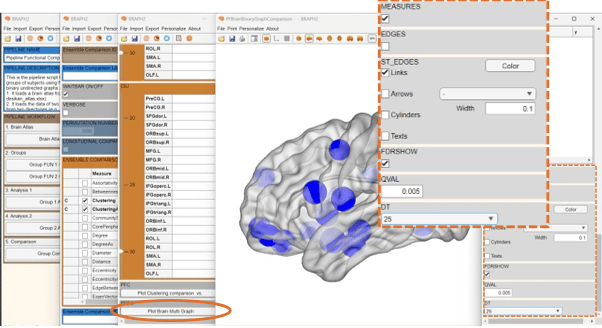
Figure 16. Regions that are significant after applying FDR at a q_value = 0.005.
We can also plot the results of global measure (in this case, ClusteringAv) from the comparison by pressing “Plot ClusteringAv comparison vs.” in the measure’s table GUI (Figure 17). In this plot we can see the differences in global clustering values between the groups at each density (Orange points). The lines from the black points indicate the upper and lower confidence intervals.
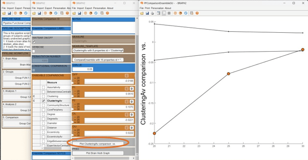
Figure 17. Plotting global measure.