GUIfMRIGraphAnalysisWU is a graphical user interface that allows the user to perform a brain graph analysis of fMRI data using weighted undirected graph (WU = Weighted Undirected). The user can calculate group measures, compare them with random graphs, and compare the measures of two groups by permutation test. Significance intervals and single/double-tailed p-values are provided (the p-values can be corrected for false discovery rate (FDR) in the case of nodal measures). Global and nodal measures are displayed separately; for nodal measures the user has the option to visualize the results on a brain surface. The graph analysis can be saved in a file *.fga for future use within BRAPH; it can also be exported in xml format for use within other programs.
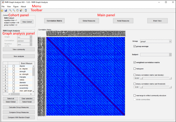
The layout of GUIfMRIGraphAnalysisWU is shown in figure 1. It is composed of five main work areas:
- Menu permits one to access the basic functionalities of GUIfMRIGraphAnalysisWU, including loading and saving an fMRI graph analysis.
- Toolbar gives direct access to some of the most commonly employed functionalities, in particular loading and saving an fMRI graph analysis.
- Cohort panel permits one to view the fMRI cohort properties.
- Graph analysis panel permits one to choose which measures to calculate or compare, view the community structure, and, if needed, start a new graph analysis.
- Main panel allows one to view the connectivity matrix as well as the calculated global and nodal measures and comparisons.
As a first example of the use of GUIfMRIGraphAnalysisWU, we will proceed to calculate some global (average strength, diameter) and local (strength, triangles) measures, and to compare the results for two groups. Then, we will visualize these results on the brain surface. Finally, we will save the graph analysis in a *.fga file.
- In the graph analysis view, select from the list of measures the average strength, diameter, strength, and triangles measures.
To quickly select more than one measure, use the buttons below the measure list:- Select all selects all the measures.
- Clear selection clears the current selection.
- Select Global selects all global measures.
- Clear Nodal selects all nodal measures.

Figure 2: Interface to calculate group measures.
- Push Calculate Group Measures in the graph analysis panel (figure 1) to calculate the selected measures. This opens a new interface, shown in figure 2. On the left of the interface, there is a list with the selected measures to be calculated. On the right, there is a popup menu to select the group for which the measures will be calculated. The calculation is started by pushing Calculate measures. When the calculation is in progress, the status of the button changes to stop and pushing it stops the calculation; the calculation can then be resumed by pressing Resume.

Figure 3: Interface to calculate group measures normalized by comparison with random graphs. - Push Compare with Random Graph in the graph analysis panel (figure 1) to calculate measures that are normalized by the results obtained from random graphs. This opens the interface shown in figure 3. This interface is analogous to that to calculate group measures, which we have seen in the previous step, but two new parameters can be inputted:
- random matrix no. sets how many random graphs are used in the comparison.
- random swaps no. sets how many times each edge is rewired to randomize the original graph.

Figure 4: Interface to compare the measures of two groups.
- Push Compare Group Measures in the graph analysis panel (figure 1) to compare the measures between two groups. This opens the interface shown in figure 4. This interface is analogous to that to calculate group measures, but with two new parameters:
- permutation number sets how many permutations are performed in the permutation test.
- longitudinal sets whether the comparison is done for longitudinal data.

Figure 5: Global measures tab.
- Push Global Measures in the main panel to visualize the results for the global measures (figure 5).
If the measure checkbox is checked, group measures are displayed (the measure and the group are selected using the popup menus at the bottom). If the comparison checkbox is checked, comparisons between two groups are displayed (the measure and the groups are selected using the popup menus at the bottom). If the random comparison checkbox is checked, measures normalized by comparison with random graphs are displayed (the measure and the group are selected using the popup menus at the bottom). By default the group average checkbox is checked; the results shown are averaged over all group subjects. To view the measure for each subject separately, uncheck this checkbox and select the subject from the neighboring popup menu.The main panel shows a table view that displays the numerical information about the selected measure. Among other data, this includes the value of the measure and the group for which it was calculated. If it is a comparison between groups or with random graphs, the difference between the values and the single/double-tailed p-values are also displayed. A series of options are available below the table view:- Select all selects all the measures.
- Clear selection clears the current selection.
- Remove removes the selected measure.

Figure 6: Nodal measures tab.
- Push Nodal Measures in the main panel to visualize the results for nodal measures (figure 6). This interface is very similar to that explained above for the global measures. The main difference is that now it is possible to select also the brain region.

Figure 7: Visualization of the brain graph on the brain surface. - Push Brain View in the main panel to visualize the nodal measures on a brain surface. By pushing the buttons at the bottom of this panel, the user can visualize the brain graph, the group measures, the comparisons between two groups, and the comparisons with random graphs.
- View brain graph visualizes the brain graph, as shown in figure 7. The graph parameters that can be specified are:– fix density draws the binary brain graph with the selected density of connections. The density can be specified by entering the value in the corresponding field or by using the slider.
– fix threshold draws the binary brain graph with all connections having larger weight than the given threshold. The threshold can be specified by entering the value in the corresponding field or by using the slider.
– weighted plots all the connection of the weighted brain graph. The weight of the connections can be encoded by color and/or thickness (by checking the corresponding checkboxes).
– Show shows the current graph on the brain surface.
– Hide hides the current graph from the brain surface.
– Color plots the current graph in the specified color.
– Set thickness sets the thickness of the connections.
Figure 8: Visualization of the nodal measures on the brain surface. - View group measures visualizes the nodal measures calculated for a given group, as shown in figure 8.[1] The group for which the measures are to be shown is selected from the popup menu in the top left. The list on the left shows the measures that have been calculated.

Figure 9: Visualization of the comparison between two groups on the brain surface. - View comparison visualizes the comparison between two groups, as shown in figure 9. The two popup menus on the left specify the two groups that are compared and the list below them shows the measures for which they have been calculated. The other functionalities are analogous to the interface for viewing group measures with two new options:– fdr (1-tailed), if checked, corrects the p-values for single-tailed false discovery rate. Only brain regions with significant p-values are then shown on the brain surface.
– fdr (2-tailed), if checked, corrects the p-values for double-tailed false discovery rate. Only brain regions with significant p-values are then shown on the brain surface.
Figure 10: Visualization of the measures normalized by random comparison on the brain surface. - View random comparison visualizes the measures normalized by comparing them with random graphs, as shown in figure 10. All the functionalities of this interface are analogous to those of the interface to visualize a comparison between groups.
- Select File
Save to save the fMRI graph analysis WU as a *.fga file; alternatively you can also use the shortcut Ctrl+S or the Save icon on the toolbar.
- Select File
- View brain graph visualizes the brain graph, as shown in figure 7. The graph parameters that can be specified are:– fix density draws the binary brain graph with the selected density of connections. The density can be specified by entering the value in the corresponding field or by using the slider.
Additional information
Cohort panel
The cohort is already uploaded when GUIfMRIGraphAnalysisWU is launched. The cohort view shows the cohort’s properties including name, number of subjects, and groups. Moreover, all cohort’s properties can be viewed in the GUIfMRICohort interface with restricted access by pushing View Cohort.
Graph analysis panel
The graph analysis panel shows the information relative to the graph analysis and gives the user the ability to calculate measures. The available features are:
- Graph analysis properties. These three popup menus show the properties of the graph analysis: graph type, correlation type, and how to deal with negative correlations. As all these properties were set in GUIfMRIGraphAnalysis, here all the popup menus are disabled and the properties cannot be changed. If the user wishes
to change any of the properties, a new graph analysis should be started. - View community opens the interface to view the community structure that is set. Also the community structure cannot be changed.
- New analysis opens a new GUIfMRIGraphAnalysis interface where a new graph analysis with different parameters can be launched.
- Measure list lists all measures available for calculation for weighted graphs. The user can choose which measure to calculate by checking the checkboxes next to them.
- Calculate Group Measures opens an interface allowing the user to set parameters to calculate the selected measures.
- Compare Group Measures opens an interface allowing the user to set parameters to compare the selected measures between two groups.
- Compare With Random Graphs opens an interface allowing the user to set parameters to compare the selected measures with random graphs.
Main panel
The main panel consists of a main table that displays different information about the graph analysis and the calculated measures. The console buttons are used to switch between the various types of information shown in the table. The following information can be displayed:
- Correlation Matrix visualizes the connectivity matrix based on the parameters set on the right. For more detailed information about how to visualize the connectivity matrix please refer to the section Main view in the chapter fMRI Graph Analysis.
- Global Measures allows the user to visualize global measures.
- Nodal Measures allows the user to visualize nodal measures.
- Brain View allows the user to visualize the brain graph and the calculated nodal measures on a brain surface.
Menu
File provides various options for importing and saving an fMRI graph analysis WU:
- File
Open (Ctrl+O) opens a popup window to load an fMRI graph analysis WU saved in *.fga format.
- File
- File
- File
- File
- File
View switches the main view to display various types of information:
- View
- View
- View
- View
Figure
About
Toolbar
The toolbar provides different options to open and save the fMRI graph analysis WU and visualize the figures. It is shown in figure 11.

Open and save commands
These commands allow the user to open and save an fMRI graph analysis WU in the *.fga format. These are equivalent to the open and save menu options in the File menu.
![]() opens a popup window to load an fMRI graph analysis WU saved in *.fga format.
opens a popup window to load an fMRI graph analysis WU saved in *.fga format.
![]() saves the current fMRI graph analysis WU in *.fga format.
saves the current fMRI graph analysis WU in *.fga format.
Visualization commands
These commands allow the user to control the visualization of the graphical representations.
![]() zooms in image.
zooms in image.
![]() zooms out image.
zooms out image.
![]() drags image.
drags image.
![]() shows/hides data cursor.
shows/hides data cursor.
![]() standard 3D view.
standard 3D view.
![]() sagittal left view.
sagittal left view.
![]() sagittal right view.
sagittal right view.
![]() axial dorsal view.
axial dorsal view.
![]() axial ventral view.
axial ventral view.
![]() coronal anterior view.
coronal anterior view.
![]() coronal posterior view.
coronal posterior view.
![]() switches brain surface on/off.
switches brain surface on/off.
![]() switches axis on/off.
switches axis on/off.
![]() switches grid on/off.
switches grid on/off.
![]() switches brain region symbols on/off.
switches brain region symbols on/off.
![]() switches brain regions spheres on/off.
switches brain regions spheres on/off.
![]() switches brain region labels on/off.
switches brain region labels on/off.
Footnotes and references
- ^ For more information about the rescaling and the filters needed to be applied to visualize the data, refer to the Main panel subsection in the chapter MRI Cohort.