Measure List

A graph consists of a series of nodes connected by edges. The edges can be either weighted ( ${\bf W}$ ), in which case they are associated to a real number that indicates the strength of the connection, or binary ( ${\bf B}$ ), in which case they are either 0 (absence of connection) or 1 (existence of connection). Furthermore, the edges can be either directed ( ${\bf D}$ ), if the connections have a directionality (e.g. node $j$ can be connected to node $k$ but not viceversa), or undirected ( ${\bf U}$ ), if the connections do not have a preferential directionality (i.d. if node $j$ is connected to node $k$ , then automatically node $k$ is connected to node $j$ ). The connections of a graph can be efficiently represented with a connectivity matrix, where the $j$ th row represents the out-going connections from node $j$ and the $k$ th column represents the in-coming connections to node $k$ . U graphs are symmetric. Typically, the diagonal elements of the connection matrix are set to 0, i.e. a node is not connected to itself.

Graph measures can be classified within two broad categories:

global measures refer to global properties of a graph and, therefore, consist of a single number for each graph;
nodal measures refer to properties of the nodes of a graph and, therefore, consist of a vector of numbers — one for each node of the graph.

Furthermore, we will indicate to which kind of graph a given measure belongs by using $\textbf{W}$ (= weighted graphs) or $\textbf{B}$ (= binary graphs) and $\textbf{D}$ (= directed graphs) or $\textbf{U}$ (= undirected graphs). If no letter is indicated it means that the measure applies to both cases.

Degree

Degree (nodal): Total number of edges connected to a node.

Average degree (global): Average of the degrees of all nodes.

In-degree (nodal, D): Number of inward edges going into a node.

Average in-degree (global, D): Average of the in-degrees of all nodes.

Out-degree (nodal, D): Number of outward edges originating from a node.

Average out-degree (global, D): Average of the out-degrees of all nodes.

degree

Figure 1: Degree of a node. The red node has a high degree (i.e. a large number of connections) while the blue node has a low degree (i.e. a low number of connections).

Methodological notes: For BU graphs, the degree is calculated as the sum of the number of connections across the rows or columns of the connectivity matrix. For BD graphs, the in-degree is calculated as sum over columns, while the out-degree is calculated as sum over the rows; the degree is the sum of in-degree and out-degree. For W graphs, the weights of the connections are ignored in the calculations by binarizing the connectivity matrix so that only edges with nonzero weights are considered connected.

Strength

Strength (nodal, W): Sum of the weights of all edges connected to

a node [1].

Average strength (global, W): Average of the strengths of all nodes.

In-strength (nodal, WD): Sum of the weights of inward edges going into a node.

Average in-strength (global, WD): Average of the in-strengths of all nodes.

Out-strength(nodal, WD): Sum of the weights of outward edges originating from a node.

Average out-strength (global, WD): Average of the out- strengths of all nodes.

strength

Figure 2: Strength of a node. Despite having less connections, the red node has a higher strength (only one connection with high strength), while the blue node has a lower strength (it has 7 connections, each with strength of only 0.1).

Methodological notes: For WU graphs, strengths are calculated as sums over either rows or columns of the weighted connectivity matrix. For WD graphs, in-strengths (out-strengths) are calculated as sums over columns (rows), and strengths are calculated as sums of in-strengths and out-strengths.

Eccentricity

Eccentricity (nodal): Maximal distance between a certain node and any other node [2].

Average eccentricity (global): Average of the eccentricities of all nodes.

In-eccentricity (nodal, D): Maximal incoming distance from all other nodes to a node.

Average in-eccentricity (global, D): Average of the in-eccentricities of all nodes.

Out-eccentricity (nodal, D): Maximal outgoing distance from a node to all other nodes.

Average out-eccentricity (global, D): Average of the out- eccentricities of all nodes.

Radius (global): Minimum eccentricity of all nodes.

Diameter (global): Maximum eccentricity of all nodes.

eccentricity

Figure 3: Distance between nodes. The distance between the two green nodes is the shortest possible path between them, (e.g. the red path). Other longer paths between the two nodes can also exist (e.g. the blue path).

Methodological notes: The distances (the shortest path lengths) between a node and any other node in the graph can be calculated and stored in a distance matrix. The eccentricity for a node is maximum of all distances calculated for this node. For D graphs, the in-eccentricity (out-eccentricity) is calculated as the maximum along columns (rows) of the distance matrix, the eccentricity is the larger value of the the in-eccentricity and out-eccentricity. For disconnected nodes, the eccentricity is set to NaN.

Path Length

Path length (nodal): Average distance from a node to all other nodes.

Characteristic path length (global): Average of the path lengths of all nodes.

In-path length (nodal, D): Average distance from all other nodes to a particular node.

Characteristic in-path length (global, D): Average of the in-path lengths of all nodes.

Out-path length (nodal, D): Average distance from a particular node to all other nodes.

Characteristic out-path length (global, D): Average of the out-path lengths of all nodes.

Methodological notes: The distance between two nodes is defined as the length of the shortest path between those nodes (figure 3). For B graphs, the length of a path is the number of edges. For W graphs, the length of an edge is a function of its weight; typically, the edge length is inversely proportional to the edge weight because a
high weight implies a shorter connection [3]. For D graphs, the path length of a node is the average of its in- and out-path lengths. The shortest path lengths between all pairs of nodes can be found using Dijkstra’s algorithm on W graphs and using breadth-first search on binary graphs [4].

Triangles

Triangles (nodal): Number of neighbors of a node that are also neighbors of each other [5].

triangles

Figure 4:Triangles around nodes. The red node has a high number of triangles (only the red edges contribute as the black edges are not connected between themselves), while the blue node has a low number of triangles (only 1 triangle is formed by the blue edges).

Methodological notes: For BU graphs, given a connection matrix $A$ , the number of triangles is the diagonal of $A^3$ divided by two. For WU graphs, a contribution of the triangles around the node is defined as the geometric mean of the weights of the edges forming the triangle; it can be calculated by taking each element of the connection matrix to the power of $1/3$ and the diagonal entries of the third power of the resulting matrix divided by two. For D graphs, we will consider that there is a triangle only if the directed edges between the three nodes (vertices of the triangle) are arranged so that they form a closed cycle (but other conventions are also possible.

Clustering Coefficient

Clustering coefficient (nodal): Fraction of triangles present around a node [6].

Clustering coefficient (global): Average of the clustering coefficients of all nodes.

Methodological notes: The clustering coefficient is calculated as the ratio between the number of triangles present around a node and the maximum number of triangles that could possibly be formed around that node. See also triangles for how the number of triangles is calculated. For U graphs, the total number of possible triangles is calculated as $\frac{1}{2}d(d-1)$ , where d is the degree of a node. For D graphs, we consider a triangle only if the directed edges between any three nodes form a cycle; the total number of possible triangles is calculated as $d_{in}d_{out} - d_{ii}$ , where $d_{in}$ and $d_{out}$ are the in-degree and out-degree of a node, respectively, and $d_{ii}$ is the number of connections that cannot form triangles (i.e. the number of neighboring nodes that are connected with both inward and outward edges).

Transitivity

Transitivity (global): The ratio of total number of triangles to the number of (unordered) triplets in the graph.

Methodological notes: The transitivity is calculated as 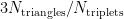$3 N_{\rm triangles}/N_{\rm triplets}$ , where $N_{\rm triangles}$ is the total number of triangles and $N_{\rm triplets}$ is the total number of triplets in the graph. $N_{\rm triplets} = \sum_i d_i(d_i-1) - d_{\rm ii}$ , where the sum runs over all nodes in the graph, $d_i$ is the total degree of each node and $d_{\rm ii}$ are the false pairs that do not result in triplets [7].

Closeness Centrality

Closeness centrality (nodal): Inverse of the path length of a node.

In-closeness centrality (nodal, D): Inverse of the in-path length of a node.

Out-closeness centrality (nodal, D): Inverse of the out-path length of a node.

Methodological notes: See path length for the calculation of the path length.

Betweenness Centrality

Betweenness centrality (nodal): Fraction of all shortest paths in the graph that pass through a node. Nodes with high values of betweenness centrality participate in a large number of shortest paths.

betweenness

Figure 5: Betweeness centrality of a node. The red node has a high betweeness centrality (many shortest paths that connect the nodes from left to right pass through the red node), while the blue node has a low betweeness centrality (no shortest path
lengths pass through the blue node).

Methodological notes: An algebraic method used to calculate the betweenness centrality is presented by Kintali [8].

Global Efficiency

Global efficiency (nodal): Average of the inverse shortest path length from a node to all other nodes [9].

Global efficiency (global): Average of the global efficiencies of all nodes.

In-global efficiency (nodal, D): Average of the inverse shortest in-path lengths of a node.

In-global efficiency (global, D): Average of the in-global efficiencies of all nodes.

Out-global efficiency (nodal, D): Average of the inverse shortest out-path lengths of a node.

Out-global efficiency (global, D): Average of the out-global efficiencies of all nodes.

Methodological notes: See path length for the calculation of the path length. After the path lengths from a node to all other nodes are calculated, they are inverted and the average gives the global eﬃciency for the node. For D graphs, the global eﬃciencies of the nodes are the average of their in- and out-global eﬃciencies.

Local Efficiency

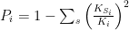
Local efficiency (nodal): Global efficiency of a node calculated on the subgraph created by the node’s neighbors.

Local efficiency (global): Average of the local efficiencies of all nodes.

Methodological notes: See global efficiency for the calculation of the global efficiency. The local efficiency is calculated by applying the same steps on the subgraph formed by the node’s neighbors. In the case of W graph, the weighted connections of the neighbors of node $i$ are calculated as $d^{\rm subgraph}_{jk} = d_{jk} \sqrt{d_{ij} d_{ik}}$ , where the nodes $j$ and $k$ are two neighbors of $i$ , and $d_{ij}$ , $d_{ik}$ and $d_{jk}$ are the weights of the edges.

Modularity

Modularity (global): Extent to which a graph can be divided into clearly separated communities (i.e. or modules). Its calculation requires a previously determined community structure.

modularity_high

Figure 6: High modularity. This graph is composed by 3 clearly separated communities with a high number of within-module connections and a low number of between-module connections.

modularity_low

Figure 7: Low modularity. This graphs is the one shown in Figure \ref{fig:modularity_high} with some extra between-module connections. The graph can no longer be clearly separated into a collection of communities.

Methodological notes: The modularity is calculated as

$\frac{1}{l}\sum_{ij} \left[ A_{ij} -\frac{k_i k_j}{l} \right] \delta_{ij}$

where $l$ is the number of edges in the graph, $A_{ij}$ represents the connectivity matrix, and $k_i$ ( $k_j$ ) is the degree of the node $i$ ( $j$ ), and $\delta_{ij}$ is $1$ if the two nodes belong to the same community and $0$ otherwise, while the sum is performed over all pairs of nodes in the graph.

Within-module z-score

Within-module z-score (nodal): Extent to which a node is connected to the other nodes in the same community. Thus, it is a within-module version of degree. Its calculation requires a previously determined community structure.

Within-module in-z-score (nodal, D): Z-score calculated only by considering the contribution of in-path lengths.

Within-module out-z-score (nodal, D): Z-score calculated only by considering the contribution of out-path lengths.

z_score

Figure 8: Within-module z-score. A node can have low z-score because it has a low number of connections (leftmost yellow node) or because it has a lot of connections outside of the community to which it belongs (rightmost yellow node). Nodes with lots of connections within their community have high z-score (e.g. violet node).

Methodological notes: The z-Score is calculated as

$Z_i = \frac{K_i - K_{S_i}}{\sigma_{S_i}}$

where $K_i$ is the degree of the node in community $S_i$ to which the node belongs, $K_{S_i}$ is the average degree of all nodes in the community $S_i$ , and $\sigma_{S_i}$ is the standard deviation of the degree of the nodes within the community $S_{i}$ .

Participation coeﬃcient

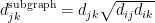
Participation coefficient (nodal): Quantifies the relation between the number of edges connecting a node outside its community and its total number of edges. Its calculation requires a previously determined community structure.

participation

Figure 9: Participation coefficient. A node has low participation coefficient if most of its connections are within its community (violet node). It has high participation coefficient if a lot of its connections are with nodes in different communities (yellow node).

Methodological notes: The participation coefficient can be calculated as

$P_i = 1 - \sum_s \left( \frac{K_{S_i}}{K_i} \right)^2$

where the sum runs over all communities, $K_{S_i}$ is the number of edges connecting the node $i$ within its community $S_i$ , and $K_i$ is the total number of edges of node $i$ . Nodes with a high participation coefficient (known as connector hubs) are connected to many communities and are likely to facilitate global intermodular integration.

Assortativity coefficient

Assortativity coefficient (global): The assortativity coefficient is a correlation coefficient between the degrees/strengths of all nodes on two opposite ends of a link [10].

Methodological notes: The assortativity is calculated as

$r = \frac{l^{-1}\sum_{i,j\in L }k_i k_j - [l^{-1} \sum_{i,j\in L} \frac{1}{2}(k_i + k_j)]^2}{l^{-1} \sum_{i,j\in L} \frac{1}{2}(k_i^2 + k_j^2) - [l^{-1} \sum_{i,j\in L} \frac{1}{2}(k_i + k_j)]^2}$

where $k_i$ and $k_j$ are the respective degrees of the nodes $i$ and $j$ , and $l$ is the number of edges in the graph. The corresponding coefficient for directed and weighted networks is calculated by using the weighted and directed variants of degree/strength. A positive assortativity coefficient indicates that nodes tend to link to other nodes with similar degree/strength.

Small-worldness

Small-worldness (global): A small-world graph has a similar characteristic path lengths as a random graph with the same degree distributio but is significantly more clustered [11].

Methodological notes: The assortativity is calculated as

$r = \frac{l^{-1}\sum_{i,j\in L }k_i k_j - [l^{-1} \sum_{i,j\in L} \frac{1}{2}(k_i + k_j)]^2}{l^{-1} \sum_{i,j\in L} \frac{1}{2}(k_i^2 + k_j^2) - [l^{-1} \sum_{i,j\in L} \frac{1}{2}(k_i + k_j)]^2}$

References

[1] Barrat, Alain, et al. “The architecture of complex weighted networks.”Proceedings of the National Academy of Sciences of the United States of America 101.11 (2004): 3747-3752.

[2] Harris, John Michael, Jeffry L. Hirst, and Michael J. Mossinghoff.Combinatorics and graph theory. Vol. 2. New York, NY, USA: Springer, 2008.

[3] Rubinov, Mikail, and Olaf Sporns. “Complex network measures of brain connectivity: uses and interpretations.” Neuroimage 52.3 (2010): 1059-1069.

[4] Kepner, Jeremy, and John Gilbert, eds. Graph algorithms in the language of linear algebra. Vol. 22. SIAM, 2011.

[5] Onnela, Jukka-Pekka, et al. “Intensity and coherence of motifs in weighted complex networks.” Physical Review E 71.6 (2005): 065103 & Fagiolo, Giorgio. “Clustering in complex directed networks.” Physical Review E 76.2 (2007): 026107.

[6] Watts, Duncan J., and Steven H. Strogatz. “Collective dynamics of ‘small-world’networks.” nature 393.6684 (1998): 440-442.

[7] Newman, Mark EJ. “Ego-centered networks and the ripple effect.” Social Networks 25.1 (2003): 83-95.

[8] Kintali, Shiva. “Betweenness centrality: Algorithms and lower bounds.” arXiv preprint arXiv:0809.1906 (2008).

[9] Latora, Vito, and Massimo Marchiori. “Efficient behavior of small-world networks.” Physical review letters 87.19 (2001): 198701.

[10] Newman, Mark EJ. “Assortative mixing in networks.” Physical review letters89.20 (2002): 208701.

[11] Watts, Duncan J., and Steven H. Strogatz. “Collective dynamics of ‘small-world’networks.” nature 393.6684 (1998): 440-442 & Humphries, Mark D., and Kevin Gurney. “Network ‘small-world-ness’: a quantitative method for determining canonical network equivalence.” PloS one 3.4 (2008): e0002051.